
The powerful capability 'Individual Physics' allows the advanced user defining his own special physical formulations, solve for them in Magnetics and exploit all the excellent tools provided by NX / Simcenter.
By using such individual formulations the user can for example put his own postprocessing equations into existing solutions. Maybe there are developed very special formulas for losses calculation depending on the B-field the user can include such formulas and get the results written into the usual NX / Simcenter plot or table result files. This capability takes advantage of the GetDP programming language that provides numerical tools as they are quickly described on this page. More documentation to GetDP can be found here.
Toolbox Multiphysics Simulation
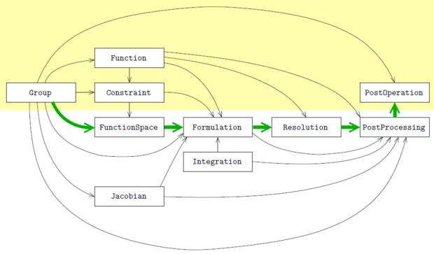
A physical problem is described by numerical objects. These objects are described in one or more text files written by the preprocessor in Magnetics for NX/Simcenter. Users who want to take advantage of individual Physics can add, remove or overwrite the default formulations.
- Group: defining topological entities
Groups result from Finite-Element-Meshes, created by the NX preprocessor. They define the topology of the problem. Every physical property that is defined in NX results in an individual group object. - Function: defining global and piecewise expressions
Using functions allows to describe material properties, constraints, loads and other data. - Constraint: specifying constraints on function spaces and formulations
They define locations with constrained degrees of freedom. - FunctionSpace: building function spaces
This object defines properties of meshes. For example the polynomial degrees of the shape functions. They also define the type of degree of freedom, e.g. node, edge, face- elements. - Jacobian: defining jacobian methods
Jacobian methods define the geometrical transformations applied to the reference elements (i.e., lines, triangles, quadrangles, tetrahedra, prisms, hexahedra, etc.). Besides the classical lineic, surfacic and volume Jacobians, the Jacobian object allows the construction of various transformation methods (e.g., infinite transformations for unbounded domains) thanks to dedicated jacobian methods. - Integration: defining integration methods
Various numerical or analytical integration methods can be referred to in Formulation and PostProcessing objects to be used in the computation of integral terms, each with a set of particular options (number of integration points for quadrature methods—which can be linked to an error criterion for adaptative methods, definition of transformations for singular integrations, etc.). - Formulation: building equations
The Formulation tool permits to deal with volume, surface and line integrals with many kinds of densities to integrate, written in a form that is similar to their symbolic expressions (it uses the same expression syntax as elsewhere in GetDP), which therefore permits to directly take into account various kinds of elementary matrices (e.g., with scalar or cross products, anisotropies, nonlinearities, time derivatives, various test functions, etc.). In case nonlinear physical characteristics are considered, arguments are used for associated functions. In that way, many formulations can be directly written in the data file, as they are written symbolically. Fields involved in each formulation are declared as belonging to beforehand defined function spaces. The uncoupling between formulations and function spaces allows to maintain a generality in both their definitions. - Resolution: solving systems of equations
The operations available in a Resolution include: the generation of a linear system, its solving with various kinds of linear solvers, the saving of the solution or its transfer to another system, the definition of various time stepping methods, the construction of iterative loops for nonlinear problems (Newton-Raphson and fixed point methods), etc. Multiharmonic resolutions, coupled problems (e.g., magneto-thermal) or linked problems (e.g., pre-computations of source fields) are thus easily defined in GetDP. - PostProcessing: exploiting computational results
The PostProcessing object is based on the quantities defined in a Formulation and permits the construction (thanks to the expression syntax) of any useful piecewise defined quantity of interest. - PostOperation: exporting results
The PostOperation is the bridge between results obtained with GetDP and the external world. It defines several elementary operations on PostProcessing quantities (e.g., plot on a region, section on a user-defined plane, etc.), and outputs the results in several file formats.
Example: Magnetostatics
Weak Formulations
Let’s have a view on the formulation object. The user can directly give the partial differential equation (PDE) of his physical problem in weak form to the system:
Maxwells equations for statics are:
curl h = j, div b = 0 and b = μh + μ0hm
h: magnetic fieldstrength,
b: magnetic fluxdensity
j: source current density,
μ: magnetic permeability
Vectorpotential form (results from div b = 0):
b = curl a
a: Vectorpotential
Weak form in classical notation (results from some algebra on the above equations):
(μ -1 curl a, curl a‘) = (j, a‘)
a‘: testfunctions
Formulation Object:
Equation{
Galerkin{ [ 1/mu[] * Dof{Curl a} , {Curl a} ]; ...};
Galerkin{ [ -j[] , {a} ]; ...}
}
It can be seen that the formulation object contains the terms of the equation. Each line contains one term.
Magnetodynamics?
Small Modification
One additional term in the formulation is needed:
Equation{ Galerkin{ DtDof[ sigma[]* Dof{a} , {a} ]; In Core; ...}; }
A new resolution for this formulation would be:
{ Name MagDyn_a_t; //time domain
System { { Name A; NameOfFormulation MagDyn_a; } }
Operation {
InitSolution[A] ;
TimeLoopTheta[0,20/50,0.1/50,1] {
tmin,tmax,dt,theta
Generate[A]; Solve[A]; SaveSolution[A];
}
}
}
For more information, please visit www.getdp.info
")
")