The magneto-dynamic solution in frequency domain describes the distribution of magnetic fields and eddy currents due to time harmonic excitation loads.

We use a quasi stationary approximation. The assumptions are applicable in cases of dimensions << wavelength. Examples are motors, transformers and frequencies from 0 Hz to a few 100 kHz.

Features

• 2D, 3D or axisymmetric Solution
• coupled with Thermal solution possible
• Outputs Plot:
  • Magnetic Fluxdensity, Magnetic Fieldstrength, Current Density, Eddy Current Losses Density, Hysteresis-, Eddy-, Excess Loss Density - steinmetz, Magnetic Potential (a-Pot).

• Outputs Table:
  • RotorBand Torque - stresstensor, Magnetic Potential on Conductors - Fluxlinkage, Voltage on Coils, Voltage on Circuits, Electrode Voltage, Electrode Current, Current on Circuits, Power on Circuits, Eddy Current Losses, Hysteresis-, Eddy-, Excess Losses, Ohm Resistance, Coil Inductivity, Phase Shift.

Examples

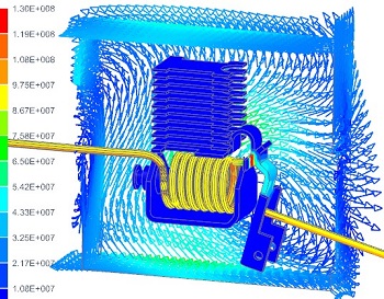
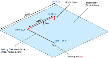
Transformer Analysis	Circuit Breaker	Lamination Losses	AC Cable

Theory and Basics

Formulations

The basis equations:
(1)        rot h = j
(2)        rot e = -δ_t b
(3)        div b = 0

Constitutive relations:
(4)        b = µ h
(5)        j = σ e

The following a-formulation is used for 2D-Magnetodynamics.

Magnetic vectorpotential a:             
(6)        b = rot a
(7)        e = -δ_t a

Magnetodynamic  weak  a-formulation:
(8)            ( µ^-1 rot a, rot a’ )_Ω
                + (-µ^-1 b_s, rot a’ ) _Ω
                        + (- j, a’ ) _ΩC
                + (σ δ_t a, a’ ) _Ωc
                        = 0, for all a’ element of Ω

The following a-v-formulation is used for 3D-Magnetodynamics.

Magnetic vectorpotential a, electric scalar potential v:             
(9)         b = rot a
(10)       e = -δ_t a – grad v

Magnetodynamic  weak  a-v-formulation:
(11)           (µ^-1 rot a, rot a’ )_Ω
                + (σ δ_t a, a’ ) _Ωc
                + (σ grad v, a’ ) _Ωc 
                + (σ δ_t a, grad v’ ) _Ωc
                + (σ grad v, v’ ) _Ωc
                      = 0

Basic Example: Team Problem 3: The Bath Plate

The problem 3 of the TEAM (Testing Electromagnetic Analysis Methods) is one of the examples for testing eddy current codes. A conductive plate with two holes is placed under a coil. The coil is driven by alternating current of 50 Hz and 1260 ampere turns. The goal is to analyze for the magnetic fluxdensity along a line that goes slightly over the plate.

The Mesh is shown in the following picture.

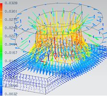
Results: Fluxdensity and  Induced Current

The magnetic fluxdensity as contourplot

The magnetics fluxdensity as vectorplot

The induced current density as contourpolot

The induced current density as vectorplot