
 The magneto-dynamic solution describes the distribution of magnetic fields and eddy currents due to time dependent
excitation loads or motion.
We use a quasi stationary approximation. The assumptions are applicable in cases of dimensions << wavelength. Examples are motors, transformers and frequencies from 0 Hz to a few 100 kHz.
Features
- 2D, 3D or axisymmetric Solution
- coupled with Thermal solution possible
- coupled with Elasticity solution possible
- Outputs Plot:
- Magnetic Fluxdensity, Magnetic Fieldstrength, Current Density, Eddy Current Losses Density, Vectorpotential, Nodal Force - virtual, Nodal Moment - virtual, Lorentz Force, Displacement
- Outputs Table:
- Total Force - virtual, Total Moment - virtual, Total Lorentz Force, RotorBand Torque - stresstensor, RotorBand Force - stresstensor, Vectorpotential on Conductors - Fluxlinkage, Voltage on Coils, Voltage on Circuits, Electrode Voltage, Electrode Current, Current on Circuits, Power on Circuits, Eddy Current Losses, Ohm Resistance, Coil Inductivity, Phase Shift.
- NVH Coupling: Forces in time and frequency domain on teeth.
- 4D Fields: Force - virtual NodeID Table, Forcedensity - virtual XYZ Table, Lorentz Force NodeID Table.
Examples
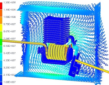
| Transformer Analysis | Circuit Breaker | Lamination Losses | AC Cable |
 |
|
 |
Theory and Basics
Formulations
The basis equations:
(1) rot h = j
(2) rot e = -δt b
(3) div b = 0
Constitutive relations:
(4) b = µ h
(5) j = σ e
a-Formulation
The following a-formulation is used for 2D-Magnetodynamics.
Magnetic vectorpotential a:
(6) b = rot a
(7) e = -δt a
Magnetodynamic weak a-formulation:
(8) ( µ-1 rot a, rot a’ )Ω
+ (-µ-1 bs, rot a’ ) Ω
+ (- j, a’ ) ΩC
+ (σ δt a, a’ ) Ωc
= 0, for all a’ element of Ω
a-v-Formulation
The following a-v-formulation is used for 3D-Magnetodynamics.
Magnetic vectorpotential a,
electric scalar potential v:
(9) b = rot a
(10) e = -δt a – grad v
Magnetodynamic weak a-v-formulation:
(11) (µ-1 rot a, rot a’ )Ω
+ (σ δt a, a’ ) Ωc
+ (σ grad v, a’ ) Ωc
+ (σ δt a, grad v’ ) Ωc
+ (σ grad v, v’ ) Ωc
= 0
Basic Example: Team Problem 1a: The Felix Cylinder
This example is a test case for electromagnetic analysis software tools. There are measured results available that will be used for comparison of our results.
The problem consists of a thin wall long hollow aluminum cylinder placed in a uniform magnetic field. The magnetic field is perpendicular to the axis of the cylinder and decays exponentially with time. The problem is to calculate the induced eddy currents at various axial positions.


Result
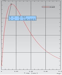
Eddy Currents over Time
The graph below shows the simulated Eddy Currents over the time.
The reference result from the team benchmark. We have to compare the Z=0.5 m curve that is responsible for the section of the tube in the middle

")
")