Der Full Wave Solver berücksichtigt alle Terme der Maxwellschen Gleichungen. Dadurch kann die Wellenlänge kleiner sein als die Abmessungen des untersuchten Teils und es sind sogar sehr hohe Frequenzen möglich. Im Frequenzbereich ergeben sich die elektrischen und magnetischen Felder aufgrund der Anregungsfrequenzen.

Features

• Plot: Magnetic Fluxdensity, Magnetic Fieldstrength, Electric Fieldstrength, Current Density, Eddy Current Losses Density, Vectorpotential, Nodal Force - virtual, Nodal Moment - virtual, Lorentz Force, Poynting Vector. 
• Table: Total Force - virtual, Total Moment - virtual, Total Lorentz Force, Voltage on Circuits, Current on Circuits, Power on Circuits, Eddy Current Losses, Ohm Resistance, Inductivity, Phase Shift.
• Coupled Thermal: Temperature

Examples

Waveguide Combiner

Theory and Basics

Formulations

The basis equations:
(1)        rot h = j + δ_t d
(2)        rot e = -δ_t b
(3)        div b = 0

Constitutive relations:
(4)        b = µ h
(5)        d = ε e
(6)        j = σ e

The following a-v-formulation is used for 3D

Magnetic vectorpotential a, 
electric scalar potential v:             
(7)        b = rot a
(8)      e = -δ_t a – grad v

Magnetodynamic  weak  a-v-formulation with full wave extension:
(9)            (µ^-1 rot a, rot a’ )_Ω
                + (σ δ_t a, a’ ) _Ωc
                + (σ grad v, a’ ) _Ωc 
                + (σ δ_t a, grad v’ ) _Ωc
                   + (σ grad v, v’ ) _Ωc

                + (ε δ²_t a, a’ ) _Ω 
                + (ε δ_t grad v, a’ ) _Ω 
                + (ε δ²_t a, grad v’ ) _Ω 
                + (ε δ_t grad v, grad v’ ) _Ω 

                      = 0

+Silver-Müller radiaton condition at infinity (outgoing waves)

Electric-field formulation

In case of wave guide solutions the solver uses the e-field formulation

(10)        rot rot e + σ µ δ_t e + ε µ δ²_t e = 0

The equation can be solved in the time or frequency domain.

Basic Example: Waveguide Loaded Cavity

The statement of this Team Workshop Problem 18 is to find the resonant frequency and other results of a square-shaped TE101 cavity coupled to a rectangular waveguide through a centered symmetrical inductive iris. All walls are perfectly conducting.

a = 22,86 mm
d = 2*a/8
L = 26,86 mm
t = a/32

The analysis is done in 2D and 3D. The pictures demonstrate these two meshes.

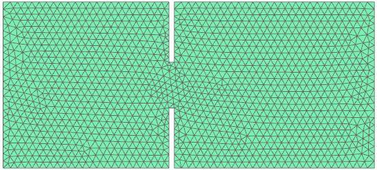
2D mesh with 2744 tri elements.

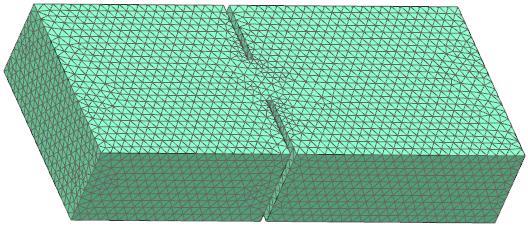
3D mesh with 38151 tetrahedral elements.

Results

Reference and Numerical Results

Reference results [1] are compared to the results of the Magnetics solution. They show a good agreement.

Reference Result: 
    Freq = 9,180 GHz

Numerical Result 2D mesh
    Freq = 9,171 GHz
    Deviation: 0,1%

Numerical Result 3D mesh
    Freq = 9,158 GHz
    Deviation: 0,24%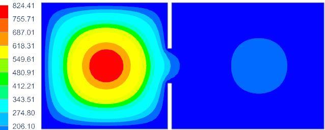


2D Result of E-Field Pattern [V/m]

Graph Maximum E-Field over Frequency

[1]: Bardi, I., Biro, O., Dyczij-Edlinger, R., Preis, K., & Richter, K. (1994b). Solution of TEAM Benchmark Problem 18 “waveguide loaded cavity”.