
 Die elektrokinetische Lösung, auch "DC Conduction Steady State" genannt, beschreibt die Verteilung des statischen elektrischen Stroms in Leitern.
Features
- 2D, 3D or axisymmetric Solution, static
- Plot: Scalarpotential, Electric Fieldstrength, Current Density, Eddy Current Losses Density.
- Table: Ohm Resistance, Electrode Voltage, Electrode Current, Eddy Current Losses.
- Coupled Thermal: Temperature.
Examples
| RJ45 Connector | 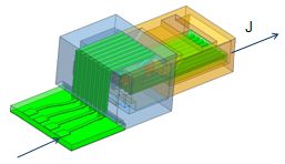 |
Theory and Basics
Formulations
The basis equations:
(1) rot e = 0
(2) div j = 0
(3) j = σ e
Boundary conditions:
(4) n x e | Γ0e = 0
(5) n * j | Γ0j = 0
Electric scalar potential formulation for the conducting region:
(6) div σ grad v = 0 with
(7) e = -grad v
Electrokinetic weak v-formulation:
(8) (σ grad v, grad v’ )Ω = 0
for all v’ element of Ω
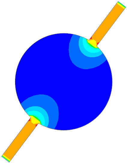
Basic Example: Ohm Resistance of Circular Plate
In this example we analyze for the ohm resistance in a circular plate. The simulated electric current density is shown in the following picture.
Results
Analytic and numerical Results
Mesh:
Elements: 5406
Nodes: 11074
Analytic Result:
R = 1.08108e-5 Ohm
Numerical Result
R = 1.069698e-5 Ohm
Deviation: 0.089%
")
")