
 Die elektrostatische Lösung beschreibt die Verteilung elektrischer Felder aufgrund statischer Ladungen und / oder elektrischer Potentiale.
Features
- 2D, 3D or axisymmetric Solution, static
- coupled with Thermal solution possible
- Outputs Plot:
- Electric Fluxdensity, Electric Fieldstrength, Electric Potential (phi-Pot)
- Outputs Table:
- Capacity, Electrode Voltage, Electrode Charge
Examples
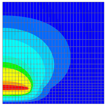
| Electrical Feedthrough |  |
Theory and Basics
Formulations
The basis equations:
(1) rot e = 0
(2) div d = ρ
(3) d = ε e
Boundary conditions:
(4) n x e | Γ0e = 0
(5) n * d | Γ0d = 0
Electric scalar potential formulation:
(6) div ε grad v = - ρ with
(7) e = -grad v
Electrostatic weak v-formulation:
(8) ( -ε grad v, grad v’ )Ω = 0,
for all v’ element of Ω
Basic Example: Point and Cylinder
Given is a charge Qf that is applied to a cylindrical face. The face starts at the position (0,0,0) has an radius of R and a length of d. Further there is another charge Q being applied to a point, that is positioned on the axis of the cylinder and has a distance of a (a>d) from the origin. The hole space around has a constant permittivity of ε.
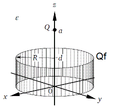
Goal is to analyze for the potential φ along the axis of the cylinder using the following parameters:
Q = 1e-9 As
Qf= 1e-7 As
a = 0.35 m
d = 0.1 m
R = 0.1 m
ε = 8.85419e-12 F/m
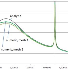
Result: Potential φ
The comparison gives good agreement between theory and numerical solution.
")
")