

In this example we want to analyse for the elastic deformations that
result from magnetic forces. A conductor is positioned in a magnetic
field resulting from two permanent magnets. In the first step, for
checking purposes we use a static magnetic solution and compare the
resulting Lorentz forces against theory.
Then, in a time domain magnetic analysis, we assign a half sinus current
running through the conductor and solve for the resulting Lorentz
forces. Such Lorentz forces on the conductor are computed for every time
step and can be post processed as graph or plot.
It follows a transient dynamic elasticity analysis to find the conductor
deformations, stresses and reaction forces. First we use the internal
elasticity solver that is delivered with MAGNETICS. Because this solver
is internally the process is very easy and fast.
Alternatively to the internal elasticity solver, we finally solve the
elasticity part by Simcenter Nastran. We apply fixed boundary conditions
and import a file that contains the Lorentz forces. As result we get
deformations and stresses.
Estimated time: 1.5 h.
Follow the steps:
download and unzip the model files for this tutorial from the
following link:
https://www.magnetics.de/downloads/Tutorials/8.CouplStructural/8.1DeformingConductor.zip
Start Simcenter, click ’Open’ and navigate to folder ’start’. Select the file ’DeformingConductor.prt’ and click Ok.
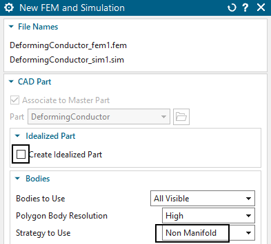
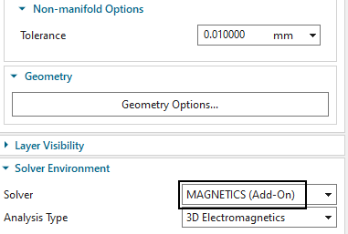
Start application Pre/Post, create a ’New Fem and Simulation’,
switch off the ’Create Idealized Part’, set the ’Strategy’ to
’Non-Manifold’, use ’Solver’ ’MAGNETICS’ and for ’Analysis Type’ use ’3D
Electromagnetics’. Click Ok.
For checking purposes, create a first Solution of Type ’Magnetostatics’ and name it ’MagSta1’.
In the Output Requests under box ’Plot’ activate ’Nodal Force - entire (virtual)’ and ’Lorentz Force (j x b)’
and under box ’Table’ activate ’Total Force - entire (virtual)’
and ’Total Lorentz Force’. Click Apply.


Background to forces: The virtual energy method is a more complete analysis of forces because it captures all such types: lorentz forces, reluctance forces and those forces that result from permanent magnets. Such completeness is not included in Lorentz forces, because Lorentz forces compute (consistent to their definition) the vector product of electric current and magnetic flux density (j x b).
In ’Time Steps’, set ’Number of Time Steps’ to 50 and ’Time
Increment’ to 0.0001 s.

Hint: The conductor has a natural frequency at 235 Hz. The electromagnetic forces will lead the conductor to vibrate in natural frequency.
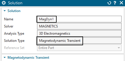
Create a second Solution of Type ’Magnetodynamic Transient’. Name it ’MagDyn1’.
Activate the same output requests as before: In box ’Plot’:
’Nodal Force - entire (virtual)’ and ’Lorentz Force (j x b)’ and in box
’Table’: ’Total Force - entire (virtual)’ and ’Total Lorentz
Force’.
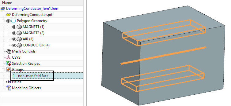
Switch to the Fem file
Optionally: Because we have used the strategy ’Non Manifold’,
check the group ’non-manifold face’ by selecting it. All faces that
belong to both air and the conductor and magnets should highlight.
Work on the conductor
Mesh the conductor using hex elements. (Tets also work). Use
’Multi Body-Infer Target’and select the front face of the conductor.
Choose the suggested element size divided by 2, and 30 layers.

Name the mesh, collector and physical ’Conductor’ and assign the
material ’Copper 5.77 e7 Siemens/meter’ (library in
NX.../SIMULATION/magnet/materials/Commonly Used Materials). Accept the
default ’Conductor Model’, ’Massive’.

Work on the magnets
Mesh the two magnets using hexa elements (tetra would also work).
Apply the material ’Samarium Cobalt: 20/30’ (library in
NX.../SIMULATION/magnet/
materials/Samarium Cobalt Permanent Magnet Materials).
To define the magnet north-direction, set the ’Magnet CSYS’ to
’Cartesian’, choose one of the csys-definition options and let the X
direction point as shown in the picture.

Optionally: Boundary layer for a perfect transition between hexa and tetra elements
The interface between tetra and hexa elements can optionally be improved. Therefore, a boundary layer with pyramid elements can be included. That layer can be only on the air side (this is what we want to do here) or it can be also on the copper side. The second case would allow detailed analysis of eddy currents. To define such a perfect transition, proceed as follows:
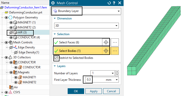
Define a ’Mesh Control’ of type ’Boundary Layer’.
Select all faces of the conductor,
activate ’Restrict to Selected Bodies’. The selection bottom ’Select Bodies(2)’ appears and two bodies are selected: The air and the conductor. Deselect the conductor because we want the transition elements only on the air.
set the ’First Layer Thickness’ to 0.3 mm. Click Ok.
Work on the air
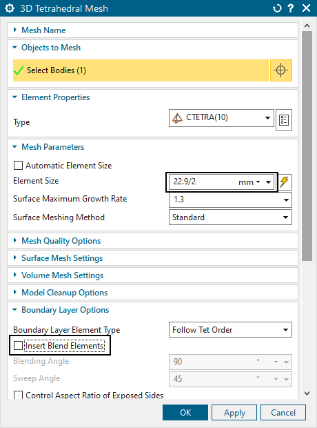
Mesh the air volume using tetra and the half of the suggested element size.
Only if the optional boundary layer mesh control is used, an
additional setting for the air mesh is available. In the setting
’Boundary Layer Options’, the checkbox for ’Insert Blend Elements’ must
be deactivated. (Otherwise the mesh may become ugly)
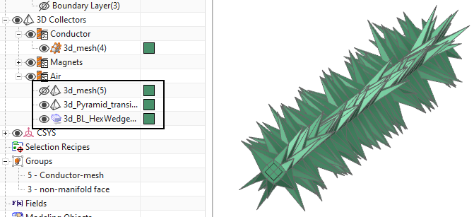
Click the ’Update’ button.
Check the newly created transition elements: Notice, there are
several new meshes created that all belong to air.
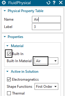
Apply a ’FluidPhysical’, activate ’Build-In’, and ’Air’ material
to ths mesh collector.


Hints: In case of mesh-mating conditions (instead of ’Non-Manifold’) the process for transition elements is a bit different: no mesh-controls are necessary. Instead, the tetra mesher would show the button ’Transition with Pyramid Elements’. If activated, a slightly simpler transition - only by one layer of pyramids - would be created.
Switch to the Sim file.
Create loads and constraints:
Create a constraint ’Flux tangent (zero a-Pot)’ on all 6 faces of
the air volume. Also apply this to the two small electrode faces of the
conductor. Apply this constraint to both solutions.


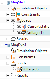
Activate the static solution and create a load of type ’Current’,
use the type ’On Solid Face’. Select one electrode face of the
conductor. Insert an ’Electric Current’ of 100 A. Name the load ’Current
static’.

Activate the dynamic solution and create a load of type
’Current’, use the type ’On Solid Face’. Select the same electrode face
as before and set the ’Method’ to ’Harmonic’. Insert an ’Electric
Current’ of -100 A, a ’Frequency’ of 235 Hz and a Phase Shift of 90 deg.
(The Phase Shift changes the default cosines type load to sinus).

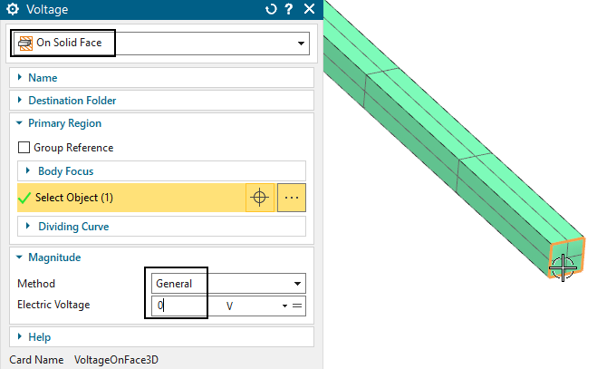
Create a load of type ’Voltage’ with 0 V, use the type ’On Solid
Face’. Select the other electrode face of the conductor. Apply this
voltage to both solutions.
Solve both solutions
Postprocess the static force results.
Open the results for the static solution and display the x component of the result ’LorentzForce’. (The same can be done for the virtual forces, witch are named ’Force’. Both results are very near)
Blank the Air mesh and all 2D meshes.
Switch from ’Contour’ to ’Arrows’.

you should see a picture like below.
Hint: Depending on your current direction the direction of the force may
be flipped.


To calculate the sum of all forces acting on the conductor you
can now compute the sum of the element forces using the ’Identify
Results’ function ![]() . Set the ’Pick’ to ’Mesh’ and select
the conductor mesh. The sum is about 0.3 N.
. Set the ’Pick’ to ’Mesh’ and select
the conductor mesh. The sum is about 0.3 N.
The analytical solution for the lorentz force on the conductor
can be found as follows:
\(\overrightarrow{F_{\mathrm{L}}}=q(\vec{v}
\times \vec{B})=I(\vec{\ell} \times \vec{B})\)
with
\(I = 100 A, B = 0.03 T, \ell = 0.1
m\)
the lorentz force results to
\(F_{L} = 0.3 N\)
Thus, the result from our simulation is close to this value.
Post process the dynamic solution as you like.
Save your parts. Don’t close them.
The internal elasticity solver can handle 3D and 1D elements. Tetra and hexa elements are by default solved by second order nodal shape functions. Instead of mid nodes the elasticity solver uses so called hierarchical shape-functions that work on the element edges and faces. With these, result quality is high and very similar to Simcenter Nastran’s second order hexa and tetra elements. Also pyramids and wedges are possible. Also, there are 1D rod and beam elements available. The solver can be used for static and transient dynamic solutions. Non-linear contacts are possible and glue conditions. Large displacement is possible as well as a strong coupling feature to electromagnetics. Currently, there is no material plasticity capability and no shell elements support. Following we set up the deforming conductor model to use this internal elasticity solver.
Set the Fem file to the displayed part.
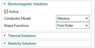
Edit the conductor physical. In box ’Elasticity Solution’, verify that ’Active’ is selected. Thus, the conductor will be solved for elasticity.
Also verify that the used material has correct values for ’Mass
Density’, ’Young’s Modulus’ and ’Poisson Ratio’: Click ’Manage
Materials’, clone the library material, rename the new one to ’Copper
EM/Mec’. In ’View’, select ’All Proporties’ and insert the ’Mechanical’
values (see picture) and use the new material for the conductor.


Check all other bodies for their setting in box ’Elasticity
Solution’. The button ’Active’ should be deactivated.


Make the Sim file to the displayed part.
Edit the static solution, in register ’Coupled Elasticity’, set the ’Elasticity Solution’ to ’Steady State’. Activate the settings as in the below picture left.
Edit the transient solution, in register ’Coupled Elasticity’,
set the ’Elasticity Solution’ to ’Transient’. Activate the settings as
in the below picture right.


Create a constraint of type ’EM Elasticity Constraint’, set the
type to ’On Edges’ and select the two edges of the conductor as shown
below. These edges will allow the conductor to deform easily because
rotation is allowed. Set all degrees of freedom to ’Fixed’, OK.


Create a second ’EM Elasticity Constraint’ on on edge of the
other side of the conductor. Fix only the x and y directions here.


Assign these two constraints to both solutions. Later we will also assign these constraints to the Nastran solution.
Solve both solutions
Post processing: The deformation (left) and von Mises stress
(right) result of the static solution are shown in the below
picture.

The maximum displacement x over time (red) and the force x (blue)
of the transient solution are shown in the below picture.

We will now extend the model for an additional Nastran transient
structural (elasticity) solution. The results will match with those from
the previous section. The key here is a file containing the node-ID
forces that will be exported from electromagnetics and inserted into
Nastran. Notice that for this method it is necessary to use the same
node-IDs in both solutions. It is possible to add meshes. It is also
possible to add mid nodes to the existing mesh for better stress results
(we will do this here). Only it is not allowed to remove nodes from the
conductor. In this case we will use a Nastran solution 402 to include
transient dynamical effects. Other Nastran solution types would also
work corresponding to their capabilities.
Advantages of using Nastran are it’s many additional capabilities (e.g.
nonlinear materials, shell elements, ...). On the other side, the
internal Magnetics elasticity solver also has advantages: the strong
coupling, large displacements and fast solutions.
Work in the Fem file:
Set the Fem file to the displayed part.
Hint: Because Nastran solutions work best with mid-node elements (Magnetics uses second order shape functions instead of mid-nodes), we switch the ’Hex’ elements against ’Hex20_compatible’. In Magnetics, such elements work identical to the conventional ’Hex’, but in Nastran, they become ’Hex20’ with mid-nodes. Proceed as follows:
Edit the conductor mesh and set the element type as in the
picture.
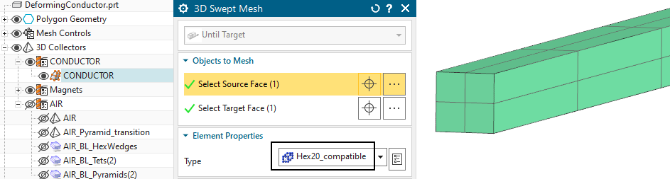
Hint: For all other element types, there exists the same compatible element type. For instance ’Tetra’ corresponds to ’Tetra10_compatible’. In this example, only the conductor must be switched because only this mesh will be used in Nastran.
Edit the Fem file and set the Solver to Simcenter Nastran,
OK.


Hint: Check the physical property of the conductor. Notice that
the type of property automatically has changed to PSOLID, because this
is now Nastran’s language. The material ’Copper EM/Mec’ is still there
and since this material has correctly defined young’s modulus, poisson
ratio and density available, it is valid also for this solver.

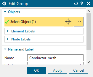
Create a group that contains only the conductor mesh. Name it
’Conductor-mesh’. Set the selection filter to ’Mesh’ and un-blank the
mesh when creating the group.
Hint: This will later be used to tell Nastran only solving for these
elements.

Switch to the Sim file.
Generate the force exchange file:
Edit solution ’MagDyn1’. In ’Output Requests’ under box ’4D Fields’, activate ’Force-virtual, NodeID Table’ and also ’Create bat-Script to convert NodeID Table to Nastran include File’. Then, at ’Cut before’ insert -0.0001 s. This setting will shift the magnetic forces by one time step. This way Nastran will activate the forces at the same time as Magnetics does. We do this only for better comparison of the two results.
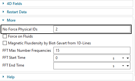
In ’More’, ’No Force Physical IDs’ enter the label of the
magnet’s physical. This is necessary to ensure that only the forces of
the conductor are transferred into the file.


Solve the solution ’MagDyn1’.
Hint: Optionally, check and verify that the results are same as before.
Hint: Notice that after the solution has finished, there is a new text file ’DeformingConductor1_sim1-MagDyn1.NodeIdForceVirt.txt’ in the working folder. This file contains the node-ID forces that will be transferred to Nastran. Notice also, there is a batch file in the same folder, named ’DeformingConductor_sim1-MagDyn1.CreateNastranInc.bat’. This batch must be executed to convert the text file into the format that can be included into Nastran.
In the working folder, double click that batch file
(’*.CreateNastranInc.bat’). There will be a file ’.inc’ created. This
inc file contains in Nastran syntax FORCE entries (and some others)
assigned to nodes and to time steps. The DLOAD ID is set to 3000, we
will use that later.


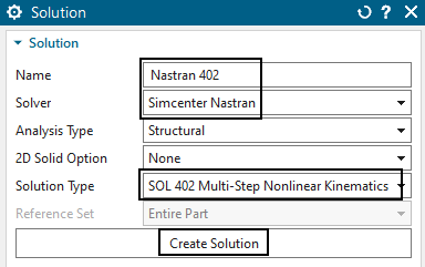
Create a usual Nastran solution:
Create a new solution of type 402 with solver Simcenter Nastran and name it ’Nastran 402’, (other transient NX Nastran solution types are also possible).
Click ’Create Solution’ then OK.
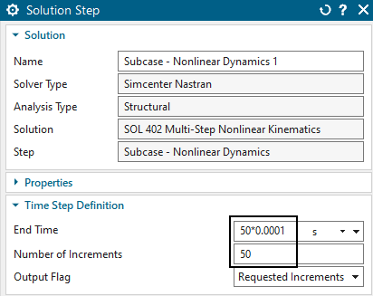
A window for the ’Solution Step’ appears. Set the ’Step’ to
’Subcase - Nonlinear Dynamics’ and click ’Create
Step’.
 Ok
Ok 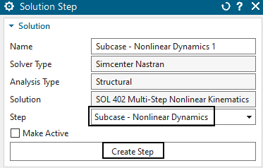
in the following window ’Solution Step’, set the ’End Time’ to
50*0.001 s and the ’Number of Increments’ to 50. Hint: we use the same
time period that we already have used in Magnetics. That could also
differ. Click OK.
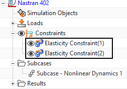
drag the two existing contraints into the Nastran solution. We simply want to reuse them.
Add the force exchange file to the Nastran solution:
Edit the solution ’Nastran 402’. In register ’Case Control’,
create a modeling object for ’User defined Text’. At ’Key in Text’
insert ’DLOAD=3000’, the force group id to be included. Optionally name
the object ’DLOAD3000’. Click Ok.


In register ’Bulk Data’, again create a modeling object for ’User
Defined Text’. Set the option ’Text From File’ to ’Linked’, click
’Browse’ and select the ’.inc’ file. Optionally name the object
’Forces-include’. Ok, Ok.


Prepare the Nastran solution
Hint: We only want to solve the conductor elements, not the magnets and not the air. Therefore, we already have created an elements group of the conductor. Following we activate a solve that only uses those elements.
Edit the solution and click ’Edit Advanced Solver options’. In register ’Export Options’ in box ’Subset Export’, activate ’Selected Groups’. From the list ’Available groups’, select group ’Conductor-mesh’ (maybe you have named it differently) and click the arrow bottom to add this group to the ’Selected groups’. Click Ok
Edit the solution again, click ’Edit Solver Parameters’ and set the ’License’ to ’Enterprise’. This is necessary because of the manually modified input file.
Click Ok.


Select the ’Solve’ buttom, deactivate ’Model Setup Check’ (because we use ’Subset Export’ the check is not allowed)
Now solve the solution
Post-processing.
For comparison of the two solvers, the picture below shows on the left two graphs of displacement (red curve: Nastran, blue: Magnetics). On the right, we see two v.Mises stress results (top: Nastran 402, bottom: Magnetics).
The deviations between the results of the two solvers are
considerably small. The small difference probably depends on slightly
different time integrations (Newmark parameters) and could be
adjusted.

to set up such a results view, proceed as follows:
Find the time step with maximum displacement. That should be step 32.
Find the node with maximum displacement. That should be node 1039.
use the feature ’Create Graph’ ![]() and create graphs of that node over time for both solutions. The two
graphs are then stored in the navigator under the corresponding
result.
and create graphs of that node over time for both solutions. The two
graphs are then stored in the navigator under the corresponding
result.
Activate ’Three Unequal Views’  to divide the window in three
parts.
to divide the window in three
parts.
insert the first displacement graph into the left view. Overlay the second displacement graph into the same.
In ’Complex Option’ choose ’Magnitude Only’.
insert the stress result of Nastran at step 32 into the right top view. Set the scale to 25 absolute (’Edit Post View’, register ’Deformation’).
insert the stress result of Magnetics at step 32 into the right bottom view. Set the scale also to 25.
Save your parts and close them.
The following method transfers transient magnetic total forces (computed on a physical body) to Nastran solutions. Special is the force transfer between different models: Meshes can be different and even 2D and 3D types can be mixed. To test this, do the following:
download and unzip the model files from the following link:
https://www.magnetics.de/downloads/Tutorials/8.CouplStructural/8.1DeformingConductor.zip
from the ’complete’ folder, open the ’DeformingConductor_sim1.sim’
Optionally, verify in solution ’MagDyn1’, ’Output Requests’, ’Table’ that total force results are active (either ’Total Lorentz Force’ or ’Total Force - entire (virtual)’)
Optionally, in register ’Coupled Elasticity’, switch off the
elasticity solution.


Solve solution ’MagDyn1’
Open the results in Post-Processing-Navigator
RMB on graph ’ForceX’ (or the corresponding name), click ’Create Table Field’ (see picture below). Repeat this for the other directions.
Check in Simulation-Navigator, Fields: A new field is created
containing time steps with force values.


In any Simcenter Nastran solution (this can also be a different Sim file or model if the fields are transferred to that), create a load of type ’Force’ (picture below),
select the whole polygon body or all his faces to apply the new force on.
at ’Force’, click the ’equal’ symbol (right in the menu) and choose ’Select Existing Field’. Then, select the newly created field.Ok
at ’Direction’, specify the corresponding direction.
repeat the load creation for the directions Y and Z.
these loads can now be used in any of the Nastran transient (or
static) solutions, for instance Sol 401/402.


The above method has been coded and extended to comfortably work on large assemblies and transient solutions. The electromagnetic model may have 3D meshes while the Nastran model may have 3D or 2D meshes. As a requirement for this transfer, all names of corresponding polygon bodies in the two models must match. This feature is available in versions NX 2306 and later. To test this, do the following:
download and unzip the model files from the following link:
https://www.magnetics.de/downloads/Tutorials/8.CouplStructural/8.1DeformingConductor.zip
from the ’complete’ folder, open the ’DeformingConductor_sim1.sim’
Optionally, verify in solution ’MagDyn1’, ’Output Requests’, ’Table’ that total force results are active (either ’Total Lorentz Force’ or ’Total Force - entire (virtual)’)
Optionally, in register ’Coupled Elasticity’, switch off the elasticity solution.
Solve solution ’MagDyn1’.
Click ’File’, ’Execute’, ’NX Open...’
Browse to the Magnetics installation folder and there into the
folder ’application’. Select the file ’EMForces2Nastran.dll’. Click
Ok.

the program now asks for an ’.afu’ file containing the forces. Select the one from the electromagnetic solution (DeformingConductor_sim1-MagDyn1__PostGraphs.afu). This file is in your working folder. Click Ok.
Hints: the program now cycles through all graphs in that file. It checks graph names: If either ’Force’ or ’LorentzForce’ is found, it extracts the force direction and the physical body name from it. For each force, the program creates
a field from that graph.
a selection-recipe that searches for a corresponding polygon-body name. From that body all faces will be selected.
Three forces for the three directions that use the selection-recipe and the field.
All newly created forces are stored in a dummy solution called
’tmp1’. From there, ’drag and drop’ them into the correct
solution.

Save your parts and close them.
The tutorial is finished.